The Taylor Series and how it proves small angle approximations!
- Michelle Ncube
- Nov 28, 2025
- 4 min read
In A level Maths, we learn that for small angles, trigonometric functions can be approximated as :
sin θ ≈ θ cos θ ≈ 1 - 0.5(θ)² tan θ ≈ θ (Where θ is in radians)
But where do these approximations stem from?
In this blog, we will cover what approximations are and why these approximations are valid.
What does it mean to approximate?
Approximating a value is essentially calculating a value that is similar or close to the true value which is easier to work with.
For example, using the sin θ ≈ θ to find sin (0.5) would give 0.5
The true value of sin (0.5) is 0.4794255386…
The approximation (0.5) gave a value very similar to the actual value despite it not being exactly 0.479. So, as they are pretty close, we can say 0.5 is an approximation for sin (0.5).
Why do we approximate values (especially in physics)?
We approximate values in physics to simplify equations so that they can become easier to solve.
Looking back at GCSE, in motion problems, you are expected to ignore air resistance as the questions usually state “air resistance is negligible” . This is not because air resistance is non existent because in the real world it is, but it’s because including it would make the problem you are trying to solve more complicated at that level.
Small angle approximations act in a similar way, instead of a number such as 0.4794255… we can use 0.5 which makes a problem become more manageable, especially when there are multiple steps and variables involved.
This may cause questions to arise, isn’t it dangerous if we are using small angle approximations such as sin (0.5) for physics problems that involve real world application.
Well no, measurements have errors etc. approximations do introduce error but if in the range they are valid, this error is extremely small. For example sin 0.1 is 0.099833…. Compared to 0.1 . As you use smaller values, the more accurate the approximation gets meaning the error is not as large as expected.
Taylor series
The Taylor series, created by Brook Taylor (a mathematician) allows for the expression of functions such as trigonometric, exponential and polynomials as an infinite sum of powers of x. This is where the approximation for small angles comes from.
For example, a function such as sin x can be written as

This works as functions such as some and cosine are continuous, meaning they are defined for every real number and can be differentiated an infinite number of times. Because of this, exapsning them into a series becomes easy.
The summation for a Taylor series of any function can be expressed in the following 2 ways:


Where:
fⁿ represents the function differentiated n times
‘a’ represents the point at which we are trying to approximate the function
2! = 2 x 1
3! = 3 x 2 x 1
n! = n x (n-1) x ….
Another way of thinking about this is basically finding an equation that matches the sin curve originating from a point (a,0).
Finding the Taylor expansion of sin x:
(Note : sin x & sin θ represent the same thing)
To calculate the approximation, knowing the differentiated versions of sin x it’s important.
If f(x) = sin x
f’(x) = cos x
f’’(x) = -sin x
f’’’(x) = -cos x
f’’’’(x) = sin x
As you can see, when function like sin x is differentiated, its derivatives repeat in a cycle between positive and negative cos x and sin x. We can use this and substitute it into the equation. Steps are shown below.


Now that we have the Taylor series of sin (x), if we substitute 0.5 into the equation, it gives an approximate value of 0.4794255332… where the real value is 0.4794255388…
This shows the that Taylor expansion is an accurate approximation of angles such as sine. If you want, you can try finding the Taylor expansion of cosine and seeing if it gives an approximate value of cos( small angle in rad).
You do not need to find the Taylor expansion for infinite powers but it’s good to know that the more terms you have in the Taylor expansion, the more accurate your approximation will be. The gallery of pictures below shows how the Taylor series for sin x looks like as you increase the number of terms.


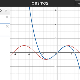


As you can see, every term added makes the expansion closer and closer to the graph of sin x, showing how the more terms we have the more accurate the approximation from the expansion is.
Using the Taylor series to justify the approximate of sin θ ≈ θ:
These are the following expansions for sine and cosine.

If we look at sine and want to find sin (0.1), substituting 0.1 into the equation will mean:
The first term is 0.1
The second term is 0.00016666….
The second term is 0.00000008333…
As you can see, the terms are getting smaller and smaller rapidly. So if we were to do:
0.1 - 0.00016666 + 0.00000008333
This would equate to 0.0998 which is approximately 0.1
Hence why sin θ ≈ θ
The same thing can be done with cosine and tangent.
Maclaurin series
This is the same as Taylor series but for points around zero zero. The reason it’s called this is because of Colin Maclaurin who popularised the use of the Taylor series around 0,0. The formula is shown below.


Because of the Taylor series and Maclaurin series we are able to approximate functions making problems easier and simpler to solve!
Further reading prompt/
Try sketching the Taylor expansion of cos x next to cos x and see how it differs as you add more terms.
Are there any other series that are useful in mathematics/physics?
Eulers identity and how you can use the Taylor series to prove it.
Sources:


Comments